Illustrative examples for a specific day

Using the data corresponding to the outputs of FLEXPART-WRF forced with ERA5 and the TROVA configuration file provided in the following repositories https://zenodo.org/records/14886887 and https://zenodo.org/records/14939160, the results shown below for October 17, 2014, can be reproduced. For this analysis, the Canary Islands are considered as the target region (magenta contour on the graphics shown). The Python codes to process these results and create the corresponding maps can be found in the repository https://zenodo.org/records/14886887.

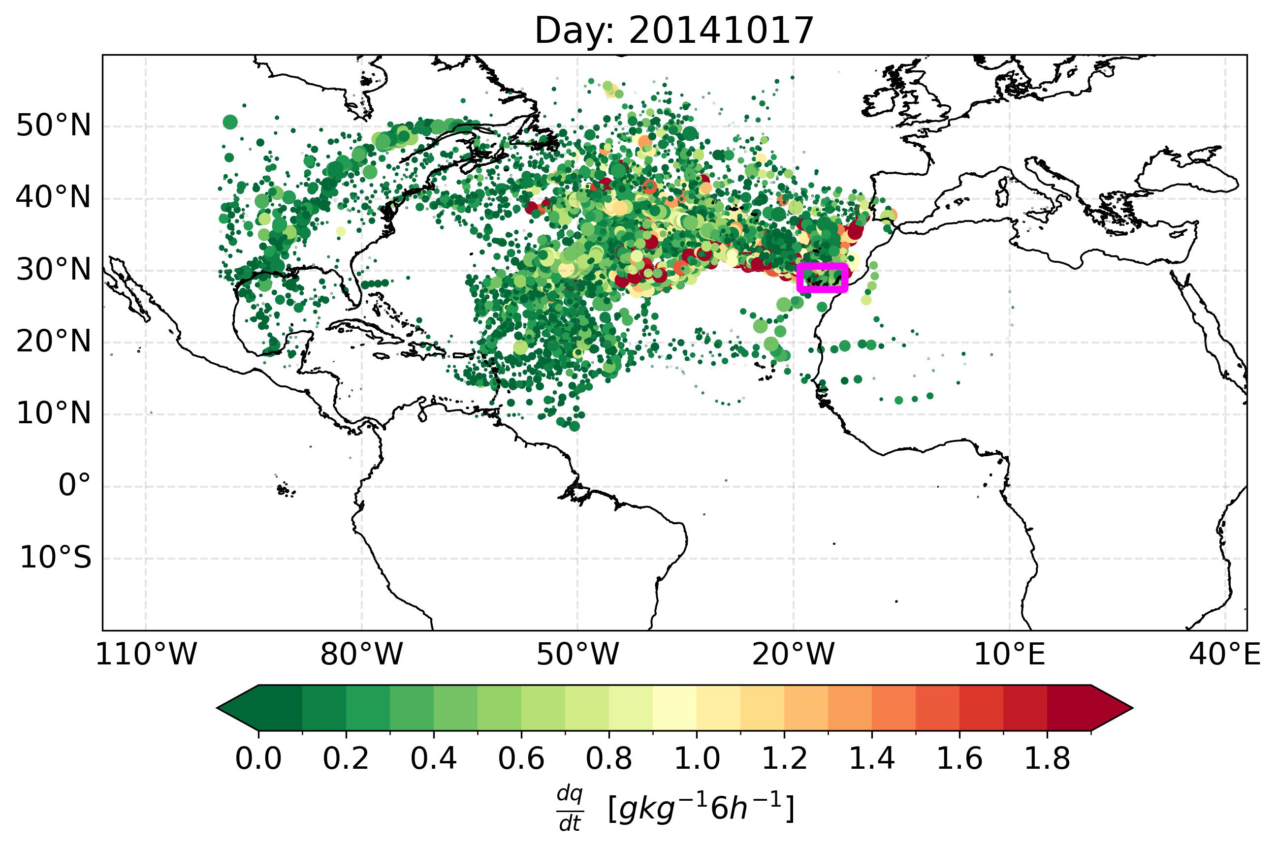
Below we show a detailed analysis of the results obtained when we ran TROVA using the methodology of Sodemann et al (2008). This analysis is performed for a sample of 1000 particles. For this analysis, we used the files 20141017000000_dqdt_back.nc and 20141017000000_back.nc. We present four figures with the following variables:

Specific humidity changes every 6 h for the particles

def plot_line_dq_dt(lat, lon, m_id, lat_id, lon_id, name, title):

   rcParams.update({'font.size': 15})
   fig=plt.figure(figsize=(10,8))
   ax1=plt.subplot(111,projection=ccrs.PlateCarree())
   ax1.add_feature(cfeature.COASTLINE.with_scale('10m'), linewidth=0.9)
   ax1.set_extent([-116,43,-20,60], crs=ccrs.PlateCarree())

   unit=r'$\frac{dq}{dt}$'  +"  "+  r'$ [g kg^{-1} 6h^{-1}]$'
   lista=np.arange(0,2, 0.1)
   cmap=plt.get_cmap('RdYlGn_r')

   boundary_norm = BoundaryNorm(lista,
                          cmap.N)

   for i in range(len(m_id[:,0])):
     index=np.where(np.isnan(m_id[i,:]))
     if len(index[0])!=0:
         index_cero=np.where(m_id[i,:index[0][0]]==0)
         if len(index_cero[0])!=len(m_id[i,:index[0][0]]==0):
            ss=plt.scatter(lon_id[i,:index[0][0]],lat_id[i,:index[0][0]],s=(m_id[i,:index[0][0]]/np.abs(np.max(m_id[i,:index[0][0]])))*40, c=m_id[i,:index[0][0]]*1000, cmap=cmap, norm=boundary_norm)
     else:
         print (np.min(m_id[i,:]), np.max(m_id[i,:]))
         ss=plt.scatter(lon_id[i,:],lat_id[i,:],s=(m_id[i,:]/np.abs(np.max(m_id[i,:])))*40, c=m_id[i,:]*1000, cmap=cmap, norm=boundary_norm)

   lat_mask, lon_mask, mask = load_mask_grid_NR("CAN.nc", "mask", "lon", "lat", 2)
   ax1.contour(lon_mask, lat_mask, mask, levels=[0.5], colors='magenta', linewidths=3.5, transform=ccrs.PlateCarree())

   plt.title("Day: "+ title)
   cb=plt.colorbar(ss,orientation="horizontal", pad=0.06,shrink=0.8, extend="both")
   cb.set_label(label=unit, size=15)
   cb.ax.tick_params(labelsize=15)
   gl = ax1.gridlines(crs=ccrs.PlateCarree(), draw_labels=True,linewidth=1, color='gray', alpha=0.2, linestyle='--')
   gl.xlabels_top = False
   gl.ylabels_left = True
   gl.ylabels_right = False
   gl.xlines = True
   gl.top_labels = False
   gl.bottom_labels = True
   gl.left_labels = True
   gl.right_labels = False
   gl.xlines = True
   paso_h=30
   lons=np.arange(np.ceil(-110),np.ceil(60),paso_h)
   gl.xlocator = mticker.FixedLocator(lons)
   gl.xformatter = LONGITUDE_FORMATTER
   gl.yformatter = LATITUDE_FORMATTER
   gl.xlabel_style = {'size': 15, 'color': 'gray'}
   gl.xlabel_style = {'color': 'black'}
   plt.savefig(name+".jpg", bbox_inches='tight', dpi = 300)
   plt.close()

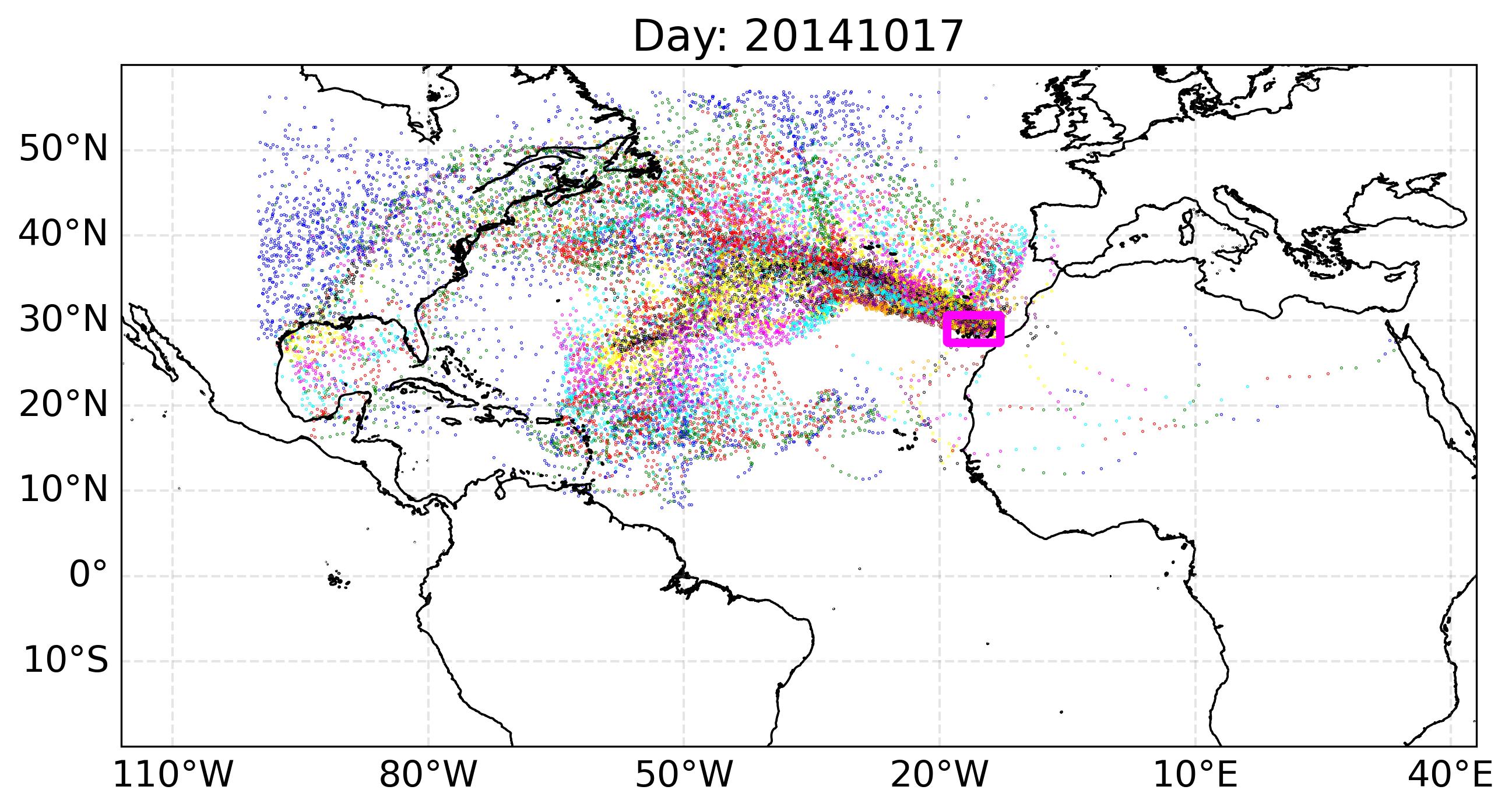
Particle positions by day shown in colors

The colors ‘blue’, ‘green’, ‘red’, ‘cyan’, ‘magenta’, ‘yellow’, ‘black’, ‘purple’, ‘orange’, ‘brown’ are associated with days from 10 to 1 in backward in time mode.

def plot_day(lat, lon, m_id, lat_id, lon_id, name, title):

   rcParams.update({'font.size': 15})
   fig=plt.figure(figsize=(10,8))
   ax1=plt.subplot(111,projection=ccrs.PlateCarree())
   ax1.add_feature(cfeature.COASTLINE.with_scale('10m'), linewidth=0.9)
   ax1.set_extent([-116,43,-20,60], crs=ccrs.PlateCarree())
   colors = ['blue', 'green', 'red', 'cyan', 'magenta', 'yellow', 'black', 'purple', 'orange', 'brown']

   for j in range(m_id.shape[0]):
      values = m_id[j, :]
      values_lat = lat_id[j,:]
      values_lon = lon_id[j,:]
      selected_intervals = [values[i:i+4] for i in range(0, len(values), 4)]
      selected_intervals_lat = [values_lat[i:i+4] for i in range(0, len(values_lat), 4)]
      selected_intervals_lon = [values_lon[i:i+4] for i in range(0, len(values_lon), 4)]
      for idx, (lon, lat, interval) in enumerate(zip(selected_intervals_lon, selected_intervals_lat, selected_intervals)):
         plt.scatter(lon, lat, color=colors[idx],s=0.05)

   lat_mask, lon_mask, mask = load_mask_grid_NR("CAN.nc", "mask", "lon", "lat", 2)
   ax1.contour(lon_mask, lat_mask, mask, levels=[0.5], colors='magenta', linewidths=3.5, transform=ccrs.PlateCarree())

   plt.title("Day: "+ title)
   gl = ax1.gridlines(crs=ccrs.PlateCarree(), draw_labels=True,linewidth=1, color='gray', alpha=0.2, linestyle='--')
   gl.xlabels_top = False
   gl.ylabels_left = True
   gl.ylabels_right = False
   gl.xlines = True
   gl.top_labels = False
   gl.bottom_labels = True
   gl.left_labels = True
   gl.right_labels = False
   gl.xlines = True
   paso_h=30
   lons=np.arange(np.ceil(-110),np.ceil(60),paso_h)
   gl.xlocator = mticker.FixedLocator(lons)
   gl.xformatter = LONGITUDE_FORMATTER
   gl.yformatter = LATITUDE_FORMATTER
   gl.xlabel_style = {'size': 15, 'color': 'gray'}
   gl.xlabel_style = {'color': 'black'}
   plt.savefig(name+"_day.jpg", bbox_inches='tight', dpi = 300)
   plt.close()

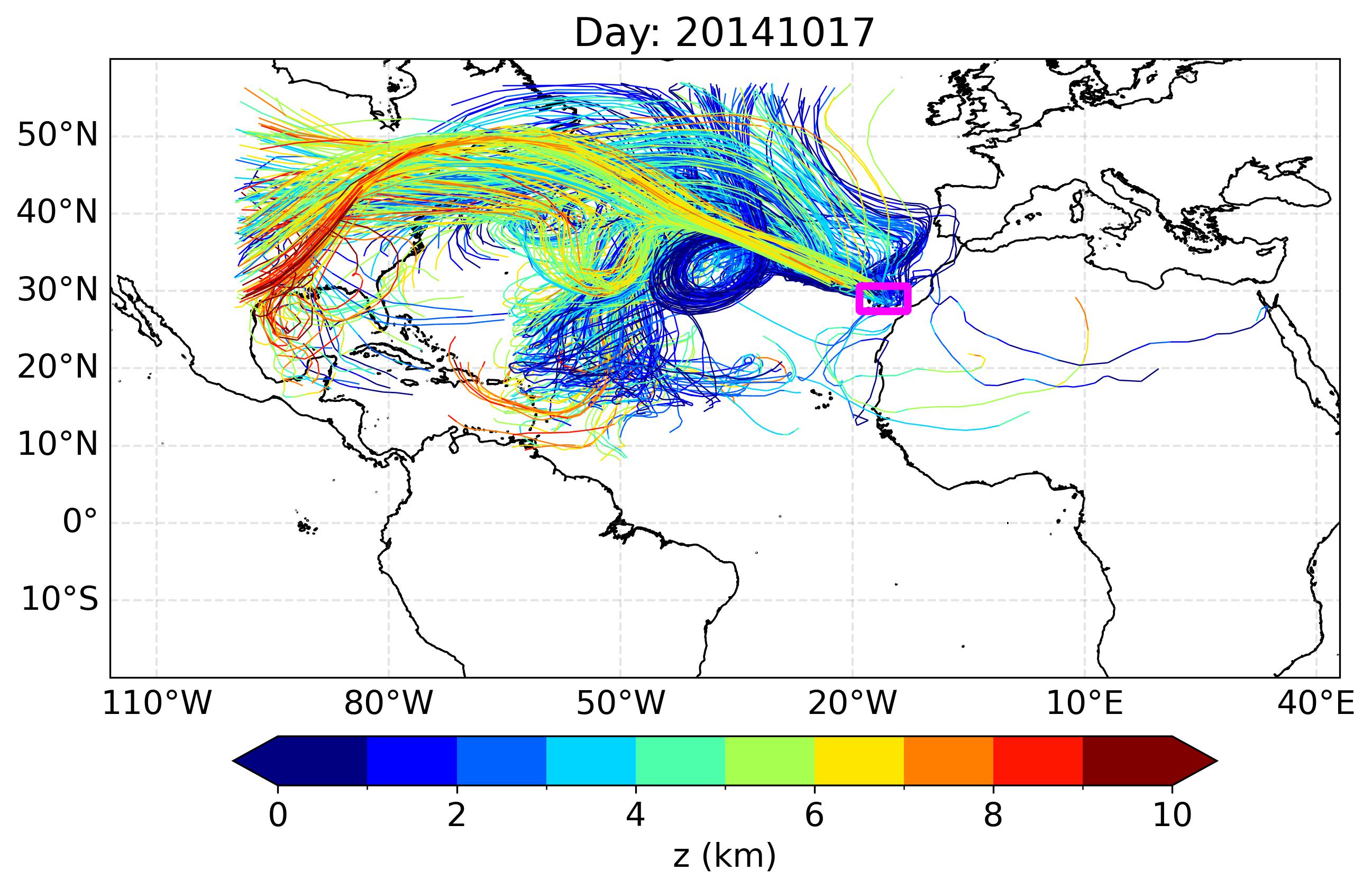
The trajectories of the particles and the height in colors every 6 h

def plot_line_z(lat, lon, m_id, lat_id, lon_id, name, title):

   rcParams.update({'font.size': 15})
   fig=plt.figure(figsize=(10,8))
   ax1=plt.subplot(111,projection=ccrs.PlateCarree())
   ax1.add_feature(cfeature.COASTLINE.with_scale('10m'), linewidth=0.9)
   ax1.set_extent([-116,43,-20,60], crs=ccrs.PlateCarree())
   unit="z (km)"
   lista=np.arange(0,10.1,1)
   cmap=plt.get_cmap('jet')
   boundary_norm = BoundaryNorm(lista,
                           cmap.N)

   for i in range(len(m_id[:,0])):
     index=np.where(np.isnan(m_id[i,:]))
     if len(index[0])!=0:
          index_cero=np.where(m_id[i,:index[0][0]]==0)
          if len(index_cero[0])!=len(m_id[i,:index[0][0]]==0):
            lc, line=colorline(lon_id[i,:index[0][0]],lat_id[i,:index[0][0]], z=m_id[i,:index[0][0]], lista=lista, cmap=cmap)
     else:
          print (np.min(m_id[i,:]), np.max(m_id[i,:]))
          lc, line=colorline(lon_id[i,:],lat_id[i,:], z=m_id[i,:], lista=lista, cmap=cmap)

   plt.title("Day: "+ title)
   lat_mask, lon_mask, mask = load_mask_grid_NR("CAN.nc", "mask", "lon", "lat", 2)
   ax1.contour(lon_mask, lat_mask, mask, levels=[0.5], colors='magenta', linewidths=3.5, transform=ccrs.PlateCarree())

   cb=plt.colorbar(lc,orientation="horizontal",pad=0.06,shrink=0.8, extend="both")
   cb.set_label(label=unit, size=15)
   cb.ax.tick_params(labelsize=15)
   gl = ax1.gridlines(crs=ccrs.PlateCarree(), draw_labels=True,linewidth=1, color='gray', alpha=0.2, linestyle='--')
   gl.xlabels_top = False
   gl.ylabels_left = True
   gl.ylabels_right = False
   gl.xlines = True
   gl.top_labels = False
   gl.bottom_labels = True
   gl.left_labels = True
   gl.right_labels = False
   gl.xlines = True
   paso_h=30
   lons=np.arange(np.ceil(-110),np.ceil(60),paso_h)
   gl.xlocator = mticker.FixedLocator(lons)
   gl.xformatter = LONGITUDE_FORMATTER
   gl.yformatter = LATITUDE_FORMATTER
   gl.xlabel_style = {'size': 15, 'color': 'gray'}
   gl.xlabel_style = {'color': 'black'}
   plt.savefig(name+".jpg", bbox_inches='tight', dpi = 300)
   plt.close()

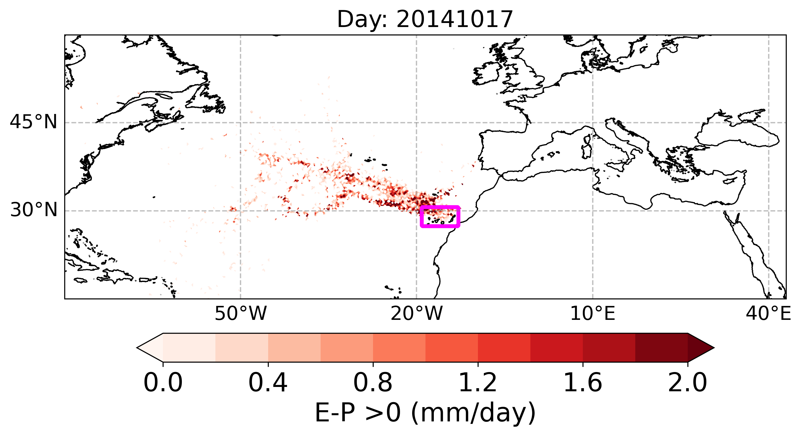
Moisture source pattern (E-P > 0)

def plot_field(lon, lat, data, name, pallete, unit, title):

   rcParams.update({'font.size': 15})
   fig=plt.figure(figsize=(10,8))

   lon, lat = np.meshgrid(lon, lat)
   ax1 = plt.subplot(111, projection=ccrs.PlateCarree())
   ax1.set_extent([-80,43,15,60], crs=ccrs.PlateCarree())
   ax1.add_feature(cfeature.COASTLINE.with_scale('10m'), linewidth=0.9)

   band_a = 0.001
   data[np.abs(data) < band_a] = np.nan
   lat_mask, lon_mask, mask = load_landmask("CAN.nc")
   unit = unit
   cf = ax1.contourf(lon, lat, data, levels=np.arange(0, 2.2, 0.2), cmap=plt.get_cmap(pallete), extend='both', transform=ccrs.PlateCarree())
   ax1.contour(lon_mask, lat_mask, mask, levels=[0.5], colors='magenta', linewidths=3, transform=ccrs.PlateCarree())

   plt.title("Day: "+ title)
   cb = plt.colorbar(cf, orientation="horizontal", pad=0.06, shrink=0.8)
   cb.set_label(label=unit, size=20)
   cb.ax.tick_params(labelsize=20)
   gl = ax1.gridlines(crs=ccrs.PlateCarree(), draw_labels=True, linewidth=1, color='gray', alpha=0.5, linestyle='--')
   gl.xlabels_top = False
   gl.ylabels_left = True
   gl.ylabels_right = False
   gl.xlines = True
   gl.xlabels_top = False
   gl.ylabels_left = True
   gl.ylabels_right = False
   gl.xlines = True
   gl.top_labels = False
   gl.bottom_labels = True
   gl.left_labels = True
   gl.right_labels = False
   gl.xlines = True
   paso_h = 30
   dlat = 15
   lons=np.arange(np.ceil(-110),np.ceil(60),paso_h)
   gl.xlocator = mticker.FixedLocator(lons)
   gl.ylocator = mticker.MultipleLocator(dlat)
   gl.xformatter = LONGITUDE_FORMATTER
   gl.yformatter = LATITUDE_FORMATTER
   gl.xlabel_style = {'size': 15, 'color': 'black'}
   gl.ylabel_style = {'size': 15, 'color': 'black'}
   plt.savefig(name + ".png", bbox_inches='tight', dpi=300)
   plt.close()

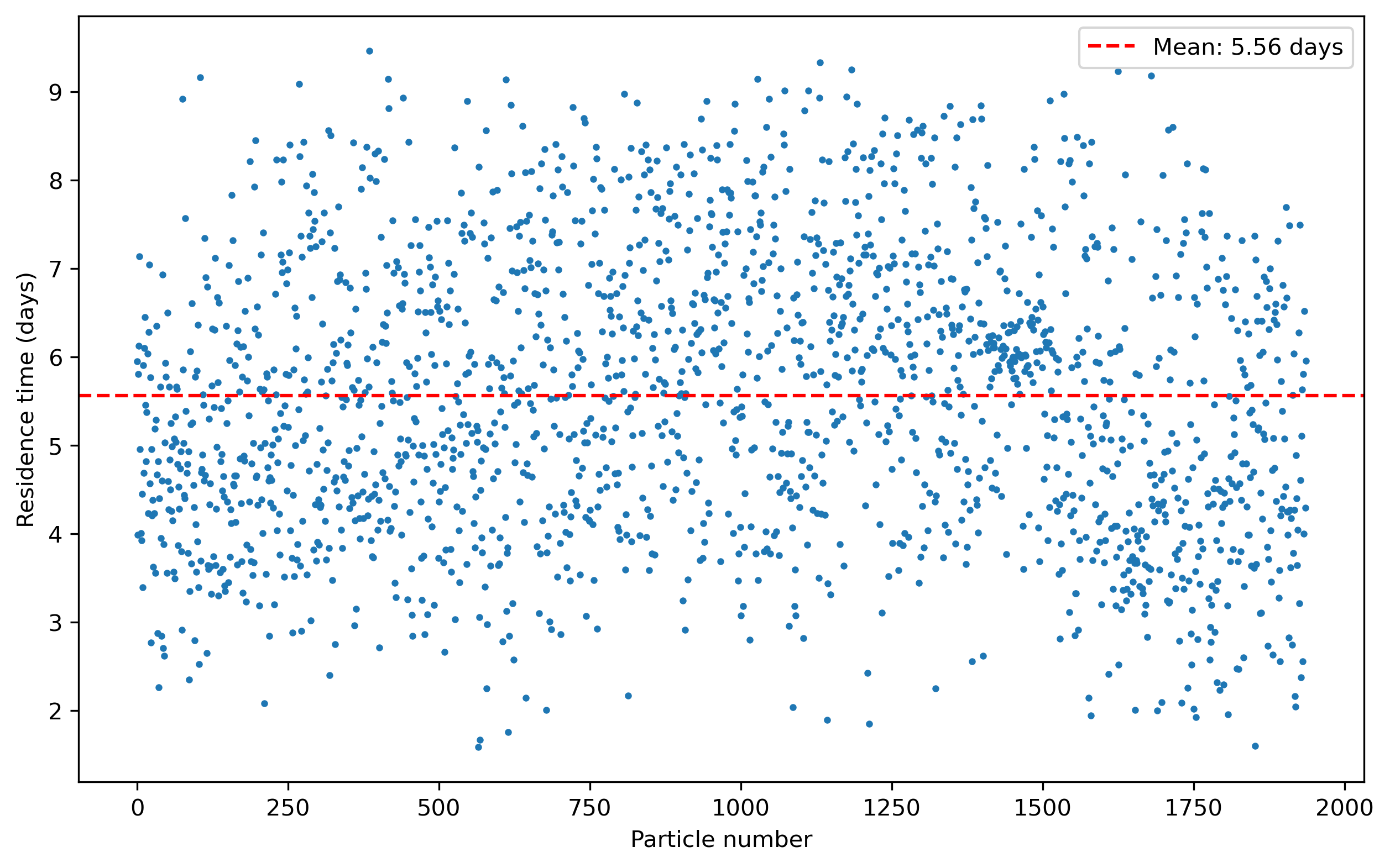
Water vapor residence time in the atmosphere

def plot_residence_time(residence_time_particles, residence_time_mean, output_dir, date, rank):

   import matplotlib.pyplot as plt
   plt.figure(figsize=(10, 6))
   plt.plot(residence_time_particles, 'o', markersize=2)
   plt.axhline(y=residence_time_mean, color='r', linestyle='--', label=f'Mean: {residence_time_mean:.2f} days')
   plt.xlabel('Particle number')
   plt.ylabel('Residence time (days)')
   plt.legend()
   plot_file = f"{output_dir}WVRT_plot_{date}.png"
   plt.savefig(plot_file, bbox_inches='tight', dpi=300)
   plt.close()
   if rank == 0:
      print("--------------------------------------------------------------------")
      print(f"Plot for the residence time for all particles saved to {plot_file}")
      print("--------------------------------------------------------------------")